ML Basics

GraphGrid Machine Learning (ML): Model Training

GraphGrid ML provides Machine Learning operations across a graph database by integrating ONgDB with Spark. Users create policies with Geequel that define their data for full machine learning pipeline management. GraphGrid ML is designed to address the following machine learning workflow:

1. Transform data
2. Train models
3. Evaluate models
4. Deploy models
5. Make predictions

ML Module Basics Tutorial Overview

In this tutorial we will explore a basic ML case study using the Iris Dataset.

1. Prepare our graph by adding the Iris Dataset in ONgDB
   • This is the data that we will train our model on.
2. Data transformation
   • We will create a transformation policy to transform our graph data so that it is formatted for ML tasks.
3. Train model
   • Train a model with a training policy.
   • The training policy is defining the pipeline stages, the training pipeline itself, and evaluation for the model
4. Inference
   • Load our model to be used to make predictions.
   • Make predictions using real-time JSON inference.

note

This tutorial requires some basic knowledge of ML to complete and understand. If you have no prior ML experience we recommend that you go over the "Machine Learning Primer" section below. If you have a good understanding of basic ML concepts you may proceed to the case study.

Machine Learning Primerß

Before we jump into the tutorial, there is some information that is integral to your success with ML. To prepare, we'll go over some general knowledge about the machine learning process.

Machine learning is about processing available data to find patterns in order to produce an algorithm that makes accurate predictions about new data. There are two sides to the ML equation: data and model architecture, both are critical to producing good predictions.

For this ML tutorial, we will only be working with labeled datasets. The goal is to transform graph data including the Iris Dataset and train a ML model with its features. We'll then use our model to make a real-time inference.

Key Terms

• Model: Represents an algorithm that has been tuned to give predictive output based on input data. Sometimes described as a "blackbox".

• Feature: single input; column (ex. Height, Weight, etc.).

• Feature Set: All the features that we're interested in.s

• Feature Vector: A datapoint; List of values that are representing a datapoint that can be trained on

• Label/Class: What we are trying to predict.

• Task: A logical namespace that helps users organize training and inference. We set a name for our task and use it throughout our policies/endpoints. A task name should describe some aspect or purpose of the work being done.

  • Our named task spans transforming, training, and inferencing with ML. A model trained in task 'A' can only be used by other task 'A' processes. Something using a task 'B' name cannot alter or use a model trained by task 'A'. For this tutorial our task will be named "predict".

tip

For example, given data with feature set {Height, Weight} we could train a model to predict if someone is an Adult. Can you predict if someone is an Adult given their feature vector [6'1", 200lbs] ?

Machine Learning Lifecycle

This is how the machine learning pipeline works:

• Transform data: Take raw graph data and transform into training data
• Train model(s): Determine steps necessary to implement desired features.
• Evaluate model(s): How well does our model preform?
• Make predictions (inferences): Use our trained model to make predictions.

Spark/MLlib

ML uses Spark's MLlib library to drive feature extraction, training, and inference. Spark is an analytics engine for data-processing at scale.

MLlib is Spark's machine learning library is used as a "training framework". This included common learning algorithms like classification, regression, and clustering; as well as common transformers and estimators like OneHotEncoding and Word2Vec.

At a high level, the library works by building "pipelines" which the data is pushed through. At each stage in the pipeline the data is either manipulated or fitted.

Transformer and Estimators

Above mentioned above, ML uses Spark's Transformers and Estimators to drive training/inference. Here is a a bit more explanation about what they are and how they work:

• Transformers: Manipulate the data

  • Things like multiplying your datapoints by a scalar, or adding additional columns to the data
  • A model is a transformer (we pass in feature vector and it transforms it into our output)
  • EX. T( x ) = x + 1

• Estimators: Try to fit the data, outputs model.

  • Algorithm that does its best to fit the data; we're approximating the data we have.
  • Output is a model that is fitted to the data.
  • EX. Linear Regression; we best fit a set of points with a line, the output is an equation. That equation is technically a transformer! We can pass new data into it and get back an estimated output value for our new data.

Real-time Inference vs. Batch Inference

ML is capable of making real-time JSON inferences for small datasets, and batch inferences for much larger datasets. This tutorial focuses on the former. Both follow the same concept. Their main jobs are to use our models to make predictions (inferences) about data.

Real-time inference is designed for running a small number of inferences and getting prediciton results directly from an endpoint. The purpose of real-time inference is to supply speedy predictons and the opportunity for data experimentation.

Instead of relying on data that is passed in through endpoints, batch inferences leverages ONgDB. This process allows batch inferences to be much more scalable and include the automatation required by certain production systems.

The key differences between real-time inference and batch inference are:

1. Batch inference sources input data from the graph while real-time inferences sources from JSON fed to an endpoint.
2. Batch inference uses a policy pattern for user customization, and has methods for monitoring and re-running inference jobs while real-time inference is run manually via an endpoint.

Case Study: Species Prediction Using Real-time Inference

For this tutorial our goal is to train our model with the Iris Dataset. This model will be able to predict iris species based on sepal and petal lengths and widths. First we need to set up the graph in ONgDB. Run this Geequel query in ONgDB to get the data we need to train on:

CALL apoc.load.csv( 'https://raw.githubusercontent.com/pandas-dev/pandas/master/pandas/tests/io/data/csv/iris.csv',  {}) YIELD list,lineNo

WITH list, lineNo
CREATE (n:Iris)
SET n += {
    `sepal_length`: apoc.convert.toFloat(list[0]),
    `sepal_width`: apoc.convert.toFloat(list[1]),
    `petal_length`: apoc.convert.toFloat(list[2]),
    `petal_width`: apoc.convert.toFloat(list[3]),
    `species`: apoc.convert.toString(list[4])
}
RETURN count(n)

Data Transformation

With our graph data in place, we can begin the data transformation process. This process is done by a transformation policy. These policies define how to get the data from the graph, and then what to do with it. The first section (source) gets raw graph data through Geequel, and specifies the return variables for later use in the policy. The second section (assignment) defines Geequel snippets that transform the source data into the format needed for training.

The assignment section is very powerful because snippets can use other snippet output as input. For example: Snippet A takes raw dates and outputs ISO8601 formatted dates, then Snippet B and Snippet C can now use A's output as input.

Transformation Policy

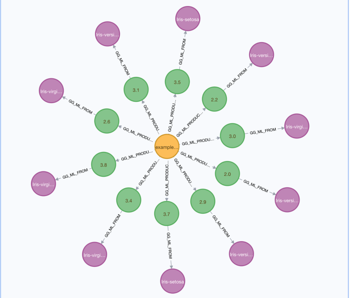
The key result of the policy is a definition of the features set in terms of snippet output. The policy also has a section (destination) that specifies how to keep track of which nodes result in which feature vectors. (A feature can be composed of data from multiple nodes!) The resulting output is a creation of a single GraphGridMLTransformation node (associated with the policy) and GraphGridMLFeature nodes that contain the extracted feature vectors.

Once we create this transformation policy we are ready to train!

Create a transformation policy using the /1.0/ml/{{clusterName}}/transformations/{mlPolicyName}} endpoint.

curl --location --request POST "${var.api.shellBase}/1.0/ml/default/transformations/transformation-policy" \
--header 'Content-Type: application/json' \
--header "Authorization: Bearer ${var.api.auth.shellBearer}" \
--data-raw '{
  "policyName": "iris-transformation-policy",
  "overwrite": true,
  "source": {
    "cypher": "MATCH (i:Iris) RETURN i.grn AS grn, i.sepal_length AS sepal_length, i.sepal_width AS sepal_width, i.petal_length AS petal_length, i.petal_width AS petal_width, i.species AS species",
    "variables": [
      "grn",
      "sepal_length",
      "sepal_width",
      "petal_length",
      "petal_width",
      "species"
    ]
  },
  "destination": {
    "nodeLabels": [
      "Iris"
    ],
    "sourceGRNs": [
      "grn"
    ]
  },
  "assignments": [
    {
      "inputs": [],
      "assignment": "apoc.text.random(1, '\''0-9'\'') + '\''.'\'' + apoc.text.random(1, '\''0-9'\'')",
      "output": "random_float_string"
    },
    {
      "inputs": [
        "random_float_string"
      ],
      "assignment": "apoc.convert.toFloat(random_float_string)",
      "output": "random_float"
    }
  ],
  "feature": {
    "grn": {
      "source": "grn"
    },
    "sepal_length": {
      "source": "sepal_length"
    },
    "sepal_width": {
      "source": "sepal_width"
    },
    "petal_length": {
      "source": "petal_length"
    },
    "petal_width": {
      "source": "petal_width"
    },
    "species": {
      "source": "species"
    }
  }
}'

Train Model

With our data transformed, the next step is to train out model. We do this with a training policy.

Training Policy

A training policy works similarly to the transformation policy. However, instead of Geequel snippets to transform data, the training policy leverages Spark to build entire machine learning pipelines. These policies have a dataFrame section that defines how to retrieve data from ONgDB, and how to change our ONgDB training data into Spark (technically Scala) types.

From there the rest of the policy is defining the pipeline stages, the training pipeline itself, and evaluation for the model. Training policies support name-bound inputs/outputs.

Uses Spark Transformers and Estimators to build pipelineStages.

The trainingPipelines then takes some (or all) of these stages and lists them in the order so that their inputs/outputs all line up.

Why does our policy define pipelineStages that aren't used in the trainingPipeline? Because estimators try to fit the data and provide a useful transformer that can be used as an input for another pipelineStage.

Parts of the Training Policy Explained

• assembler - (VectorAssembler, Transformer) constructs dataframes of our features, output is features
• kmeans - (Clustering algorithm, Estimator) implicitly uses features as default input. Produces a single prediction output or type int
• indexToString (Takes in an integer and returns a string, Transformer) - explicitly uses inputCol of prediction and the estimator provided by stringIndexerModel to map numeric model predictions to our Iris species names
• stringIndexer (Encodes strings into integers, Transformer) - uses sourceData and transforms species (our labels) into integers

Train a model using the /1.0/ml/{{clusternam}}/trainings/{{mlTask}}/{{mlPolicyName}} endpoint.

curl --location --request POST "${var.api.shellBase}/1.0/ml/default/trainings/predict/IrisPredictionModel" \
--header 'Content-Type: application/json' \
--header "Authorization: Bearer ${var.api.auth.shellBearer}" \
--data-raw '{
  "policyName": "example-training-policy",
  "overwrite": true,
  "dataFrame": {
    "name": "sourceData",
    "cypher": "MATCH (:GraphGridMLTransformation {policyName: '\''transformation-policy'\''})-[:GG_ML_PRODUCES]->(m:GraphGridMLFeature) RETURN m.`features.sepal_width` AS sepal_width, m.`features.petal_width` AS petal_width, m.`features.petal_length` AS petal_length, m.`features.sepal_length` AS sepal_length, m.`features.species` AS species",
    "schema": [
      {
        "name": "sepal_width",
        "type": "float"
      },
      {
        "name": "petal_width",
        "type": "float"
      },
      {
        "name": "petal_length",
        "type": "float"
      },
      {
        "name": "sepal_length",
        "type": "float"
      },
      {
        "name": "species",
        "type": "string"
      }
    ]
  },
  "pipelineStages": [
    {
      "name": "stringIndexer",
      "type": "StringIndexer",
      "parameters": {
        "inputCol": "species",
        "outputCol": "label"
      },
      "fit": {
        "name": "stringIndexerModel",
        "dataFrame": "{{sourceData}}",
        "outputs": {
          "indexerLabels": "labels"
        },
        "transform": {
          "name": "training",
          "dataFrame": "{{sourceData}}"
        }
      }
    },
    {
      "name": "assembler",
      "type": "VectorAssembler",
      "parameters": {
        "inputCols": [
          "sepal_length",
          "sepal_width",
          "petal_length",
          "petal_width"
        ],
        "outputCol": "features"
      }
    },
    {
      "name": "kmeans",
      "type": "KMeans",
      "parameters": {
        "k": 3
      }
    },
    {
      "name": "indexToString",
      "type": "IndexToString",
      "parameters": {
        "inputCol": "prediction",
        "outputCol": "predicted_label",
        "labels": "{{indexerLabels}}"
      }
    }
  ],
  "trainingData": {
    "dataFrame": "{{training}}",
    "trainingRatio": 0.7
  },
  "trainingPipelines": [
    "assembler",
    "kmeans",
    "indexToString"
  ],
  "evaluators": [
    {
      "type": "ClusteringEvaluator",
      "metrics": [
        "silhouette"
      ]
    }
  ]
}'

Inference

Now we can use our trained model to make predictions. The ML module is capable of real-time or batch inferences. Real-time inputs accepted from JSON (request body is data) and Geeqel (request body is Geequel that runs and the result of that query is run through inference). For this tutorial, we will be using real-time JSON inferences.

Load Model

First we need to load our model using the /1.0/ml/{{clusterName}}/inference/model endpoint. In the request body, we include the ML task name and the ML policy name.

curl --location --request POST "${var.api.shellBase}/1.0/ml/default/inference/model" \
--header 'Content-Type: application/json' \
--header "Authorization: Bearer ${var.api.auth.shellBearer}" \
--data-raw '{
    "task": "predict",
    "policyName": "IrisPredictionModel"
}'

Real-time JSON Inference

Now we can make a real-time JSON inference to test out our model using the /1.0/ml/{{clusterName}}/inference/json endpoint. In the request body we will define the schema inputs, outputs, and input data. You can change the input data to any random float value.

curl --location --request POST "${var.api.shellBase}/1.0/ml/default/inference/json" \
--header 'Content-Type: application/json' \
--header "Authorization: Bearer ${var.api.auth.shellBearer}" \
--data-raw '{
    "schema": {
        "input": [
            {
                "name": "petal_length",
                "type": "float"
            },
            {
                "name": "petal_width",
                "type": "float"
            },
            {
                "name": "sepal_length",
                "type": "float"
            },
            {
                "name": "sepal_width",
                "type": "float"
            }
        ],
        "output": [
            {
                "name": "predicted_label",
                "type": "string"
            }
        ]
    },
    "data": [
        4.5,
        1.5,
        0.3,
        0.5
    ]
}'

Prediction

Our model predicted the species of iris to be "Iris-versicolor" based on the input data. (Your prediction may be different based on your input values.)

{
    "response": null,
    "exception": null,
    "statusText": null,
    "statusCode": 0,
    "result": {
        "predicted_label": "Iris-versicolor"
    }
}

Recap

In this tutorial we transformed our graph data to a specific format needed for it to be used for ML tasks. Then we trained a model from that data and used it to make a prediction!