ML Batch Inference

GraphGrid ML provides machine learning operations across a graph database. This tutorial focuses on ML's batch inference capability. We recommend following the ML Basics tutorial before proceeding as we will be using the trained model from the ML basics tutorial. We will briefly go over the model training process, but for a full understanding of CDP's ML model training process, complete the ML Basics tutorial.

ML Batch Inference Overview

In this tutorial we will be using the Iris Dataset to perform batch inferencing with CDP's ML module. We'll train our model to make predictions about an iris plant's species using its petal and sepal measurements. To show how batch inferencing works, we'll add our own sample data to make predictions on.

1. Preliminary Steps
   a. Prepare our graph by adding the Iris Dataset in ONgDB
   • This is the data that we will train our model on.
     b. Data transformation
   • We will create a transformation policy to transform our graph data so that it is formatted for ML tasks.
     c. Train model
   • Train a model with a training policy.
   • The training policy defines the pipeline stages, the training pipeline itself, and evaluation for the model
2. Running Batch Inference
   a. Add new data to the graph to make predictions on
   b. Create a batch inference policy (BIP)
   c. Run job via the batch inference endpoint
   d. Check the status of the job and the results

Real-time Inference VS Batch Inference

CDP's ML module has two inference methods, real-time and batch. Both are for making predictions using models trained by the ML module. They are similar in concept, but have their own strengths depending on use.

If a user wants to run a small number of inferences, they should leverage real-time inference. Real-time inference is designed for speedy predictions and experimentation. User should leverage batch inference when running large jobs. This is effective for scalability and automation required by certain production systems.

We'll be using the same trained model from the ML basics tutorial to predict the species of iris plants. Recall in the previous tutorial we had to manually enter the prediction data in a json format. If you had a large dataset this would not be an efficient way to make predictions. Batch inference pulls our prediction data from ONgDB so we don't have to enter it manually.

To summarize, the main differences between real-time inference and batch inference are:

1. Batch inference sources input data from the graph, while real-time inference takes input from an endpoint.
2. Batch inference uses a policy pattern for user customization, and has methods for monitoring and re-running inference jobs. Real-time does not have these capabilities.

How Batch Inference Works

In the context of batch inference we call the set of data we want to make predictions on the "batch". A run of batch inference processes a single batch. The actual contents of a batch are customized by the user for their specific models and needs.

Tasks and Jobs

Tasks

A task is a logical namespace that helps users organize training and inference. We set a name for our task and use it throughout our policies/endpoints. A task name should describe some aspect or purpose of the work being done. For example we will use our trained model to make a prediction so we will name our task predict.

We use named tasks during transforming, training, and inferencing with ML. A model trained in task 'A' can only be used by other task 'A' processes. Something using a task 'B' name cannot alter or use a model trained by task 'A'.

We chose to name our task predict to specify that our model and policies will make predictions. The task name should remain consistent through our batch inference policy creation.

Jobs

A job defines a reusable batch inference execution. As we will see later, jobs are stored as nodes on the graph. New jobs can be created and existing jobs can be re-run or deleted.

Jobs are uniquely identified by (1) task name, (2) policy name, and (3) jobId (creation timestamp).

Job States

A batch inference job has five total sequential states (steps):

State	Step #	Description
INITIALIZED	(0)	ML acknowledges the batch inference job request.
MODEL_LOADED	(1)	The trained ML model has been loaded succesfully.
DATA_LOADED	(2)	The batch of graph data has been loaded succesfully.
RESULTS_GENERATED	(3)	Predicitons have succesfully run on the data.
RESULTS_UPLOADED	(4)	Job results have been written to file storage (minIO).
RESULTS_WRITTEN	(5)	Inference results have been executed through the batch policy outputQuery (see Batch Inference Policy).

These states describe the steps taken by a running batch inference job.

Graph Structure

The Batch inference feature only produces one type of node and no relationships. The node label is GraphGridMLBatchInference and it is the explicit representation a job.

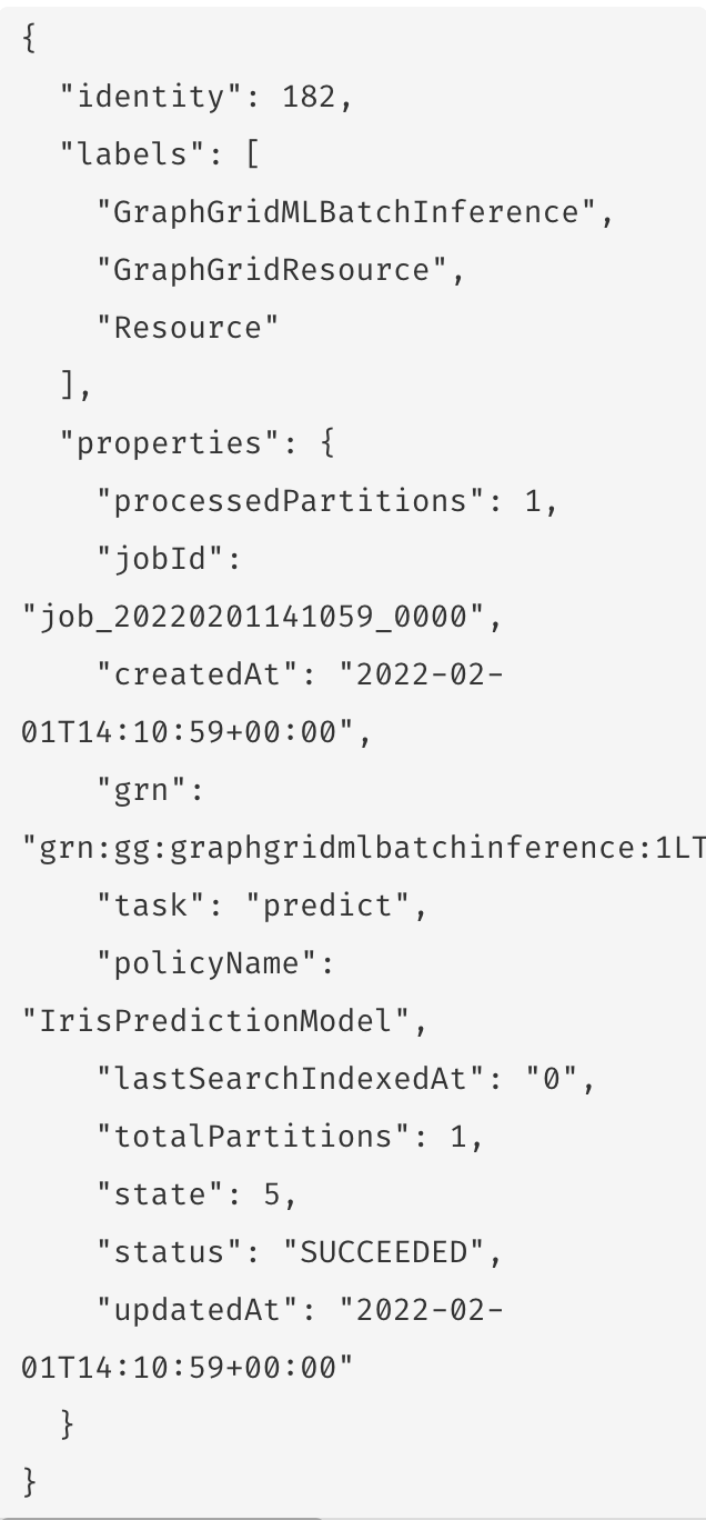
These nodes have properties for:

Property	Description
state	Which state the job is in.
status	Whether the job is running, succeded, or failed
task	Associated ML task (ex. predict)
policyName	Name of the trained model to use (must be the same policy name used to train the model).
jobId	Creation timestamp.
totalPartitions	Number of partitions formed from the original batch.
processedPartitions	Number of partitions succesfully processed.

We use the properties task, policyName, and jobId as a way to uniquely identify batch inference jobs. This trio also provides useful information about the task and exact model used for the batch inference execution.

A GraphGridMLBatchInference node represents a job and stores the jobs current state. The graph reflects real-time information about the job. Some practical uses include checking if a job has completed or using info about a failed job's last state. Jobs can be run multiple times.

Batch Inference Endpoint Operations

Batch inference is kicked off by hitting an endpoint. There are two other batch endpoints, retry batch inference and remove batch inference.

Transform Data and Train Model

We'll be using the same model from the ML Basics tutorial for our batch inference job. To continue, it is required that you to have created and trained the IrisPredictionModel from the ML Basics tutorial. If you haven't already completed that tutorial, or if you need to recreate it, head here. Once you have the trained model come back and we'll dive into batch inference!

Batch Inference

Once we have a trained model we can use it to create a batch inferencing job to predict the species of some example data that we want to run batch inference cross.

Prepare the Graph

Before we begin, add these IrisBatchInferenceTutorial nodes to the graph. These are the nodes that our batch inference job will make predictions on.

WITH [[1,5.9,3.2,4.8,1.8], [2,5.1,2.5,3.0,1.1], [3,5.4,3.7,1.5,0.2], [4,6.0,3.0,4.8,1.8], [5,4.4,3.0,1.3,0.2], [6,6.2,2.8,4.8,1.8], [7,6.4,3.2,5.3,2.3]] AS ds
UNWIND ds AS data
WITH data
CREATE (n:IrisBatchInferenceTutorial) SET n.row_id = toInteger(data[0]) SET n.sepal_length = data[1] SET n.sepal_width = data[2] SET n.petal_length = data[3] SET n.petal_width = data[4]

Batch Inference Policy (BIP)

Like many policies throughout GraphGrid CDP, the batch inference policy (BIP) is all about giving users a tool they can customize to best fit their own data. This json policy defines three important things:

1. What task and model to use and its expected input/output schema.
2. Geequel for loading data from the graph.
3. Geequel to use the resulting predictions.

Lets take a look at the example below:

{
  "task": "eventAction",
  "policyName": "example-training-policy",
  "schema": {
    "input": [
      {
        "name": "row_id",
        "type": "integer"
      },
      {
        "name": "petal_length",
        "type": "float"
      },
      {
        "name": "petal_width",
        "type": "float"
      },
      {
        "name": "sepal_length",
        "type": "float"
      },
      {
        "name": "sepal_width",
        "type": "float"
      }
    ],
    "output": [
      {
        "name": "row_id",
        "type": "integer"
      },
      {
        "name": "predicted_label",
        "type": "string"
      }
    ]
  },
  "inputQuery": {
    "cypher": "MATCH (n:IrisBatchInferenceTutorial) RETURN n.row_id AS row_id, n.petal_length AS petal_length, n.petal_width AS petal_width, n.sepal_length AS sepal_length, n.sepal_width AS sepal_width"
  },
  "outputQuery": {
    "cypher": "UNWIND ggMLResults AS ggMLResult MERGE (n:BatchInferenceResult {row_id:ggMLResult.row_id}) SET n.result=ggMLResult.predicted_label;"
  }
}

Parts of the Batch Inference Policy Explained

Task and Policy Name

Our task and policyName line up with the respective names we used to train our model. Beware, the policyName is referring to the training policy for our model and NOT the batch inference policy name.

Schema

The policy's schema maps out input and output values for our model. We've added a row_id to easily keep track of which prediction is for which datapoint.

Input Query

The input query is where the user includes their own geequel to create the batch (collect the data) to be processed. Each row the input query returns is a datapoint we will make a prediction on.

This is an example of a Geequel snippet used in an inputQuery:

 "inputQuery": {
    "cypher": "MATCH (n:IrisBatchInferenceTutorial) RETURN n.row_id AS row_id, n.petal_length AS petal_length, n.petal_width AS petal_width, n.sepal_length AS sepal_length, n.sepal_width AS sepal_width"
  }

The inputQuery collects the data that we want to make inferences on (our IrisBatchInderenceTutorial nodes) and returns it in a format that ML can use.

Output Query

What you do with the results is up to you! Whether you write them back to the graph, export them to a CSV, etc., the policy gives the user total control of how to handle results.

The outputQuery always accesses the prediction results through the variable ggMLResults. The ggMLResults variable is always a list of maps, where each map is a prediction result from our trained model.

For example, out outputQuery will write our results as BatchInferenceResult nodes.

  "outputQuery": {
    "cypher": "UNWIND ggMLResults AS ggMLResult MERGE (n:BatchInferenceResult {row_id:ggMLResult.row_id}) SET n.result=ggMLResult.predicted_label;"
  }

Run Batch Inference Job to Make Predictions

Now we'll simply use the /ml/default/inference/batch with our BIP to start a batch inference job.

curl --location --request POST "${var.api.shellBase}/1.0/ml/default/inference/batch" \
--header 'Content-Type: application/json' \
--header "Authorization: Bearer ${var.api.auth.shellBearer}" \
--data-raw '{
  "task": "predict",
  "policyName": "IrisPredictionModel",
  "schema": {
    "input": [
      {
        "name": "row_id",
        "type": "integer"
      },
      {
        "name": "petal_length",
        "type": "float"
      },
      {
        "name": "petal_width",
        "type": "float"
      },
      {
        "name": "sepal_length",
        "type": "float"
      },
      {
        "name": "sepal_width",
        "type": "float"
      }
    ],
    "output": [
      {
        "name": "row_id",
        "type": "integer"
      },
      {
        "name": "predicted_label",
        "type": "string"
      }
    ]
  },
  "inputQuery": {
    "cypher": "MATCH (n:IrisBatchInferenceTutorial) RETURN n.row_id AS row_id, n.petal_length AS petal_length, n.petal_width AS petal_width, n.sepal_length AS sepal_length, n.sepal_width AS sepal_width"
  },
  "outputQuery": {
    "cypher": "UNWIND ggMLResults AS ggMLResult MERGE (n:BatchInferenceResult {row_id:ggMLResult.row_id}) SET n.result=ggMLResult.predicted_label;"
  }
}'

And you're finished! Let ML run its magic and when the corresponding GraphGridMLBatchInference node updates its status with either "SUCCESS" or "FAILURE" you know the job is finished.

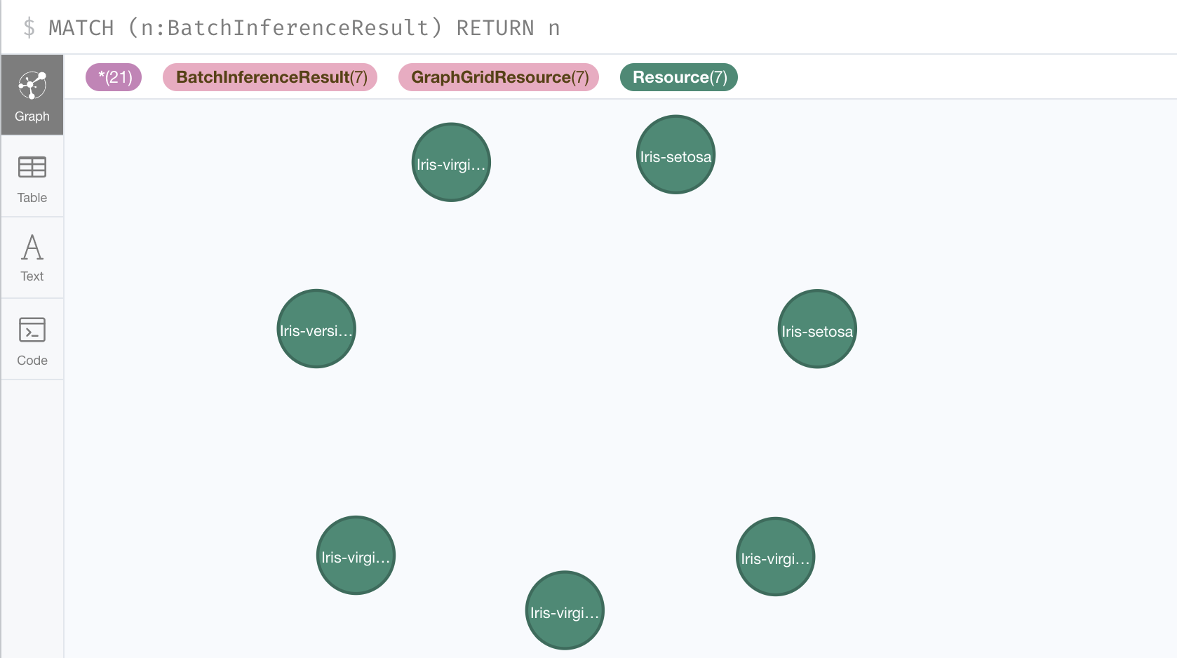
You can view the prediction results by querying the BatchInferenceResult nodes.

MATCH (n:BatchInferenceResult) RETURN n

Here we see that there are 7 BatchInferenceResult nodes contain species predictions for our 7 IrisBatchInferencetutorial nodes. Using the row_id property on the IrisBatchInferenceTutorial and the BatchInferenceResult nodes we can match our initial data to its prediction.

Conclusion

In this tutorial we used the IrisPredictionModel from the ML Basics tutorial for a batch inferencing job. We also highlighted the main differences between real-time inference and batch inference. Finally, we created a batch inference job that made predictions about the species of some data we added to the graph.